Data is the main motivation of all machine learning technic. We deal with data to find correlations and infer properties from this data. In this post, I would like to introduce the notion of a representative dataset. It was firstly proposed in the paper: “Representative datasets for neural networks”, and lately, a deeper approximation was done for the specific case of perceptrons in “Representative Datasets: The Perceptron Case”. As in the previous post, I do not pretend to do a deep explanation of these papers, just an informal taste of them.

Representative Datasets

Datasets are, nowadays, massive. Hence, the storage of this data and the time needed to process it is a problem to be solved.

Representative datasets are by definition just a subset of a dataset with some kind of closeness relation with the original dataset.

Let us be a bit more formal for a moment. A dataset is a set of pairs $(x,c)$ where $x$ is a point in $\mathbb{R}^n$ and $c$ is a label, i.e., the class where $x$ belongs. Then, we can take a subset of these pairs and if all points in the subset are close to at least one point of the full dataset, it is called representative. Besides, we consider that the definition of representative datasets should be invariant under isometric transformations of the dataset. Therefore, if there exists an isometric transformation by which the subset is representative, this subset will be considered to be representative. In the following three pictures: the first one is the original dataset, and the other two can be considered representative datasets. However, one of them is more representative than the other. In the second figure, the range of bad possible outputs of a neural network is wider than in the third figure.

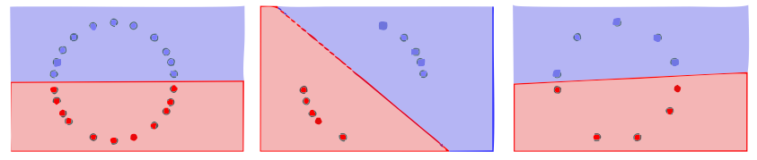
Hence we can say that all datasets are representative, but we can quantify how good is its representativeness.

In general we will have to balance how many points we erase from the full dataset and how representative is the subset. Less points in the subset will imply, in general, a worse representation of the original dataset.

How can we obtain a representative subset?

There might exist a huge range of possibilities. However, I will explain here the one in the papers we are dealing with. It is a graph approximation of the problem. Since we want to keep a closeness relation between the full dataset and the subset, we get a proximity graph with a given $\epsilon$ which is the representativeness parameter. Once we have this graph representation, we can find a dominating dataset¹, guaranteeing that each point of the subset is close to, at least, one of the full dataset. We can see this in the following picture (red points are the dominating dataset). This algorithm has complexity $O(\vert X^2\vert+\vert X\vert \vert E\vert)$.

A dominating dataset of a graph is a subset of nodes such that all of the nodes of the graph are adjacent to, at least, one node of the dominating dataset.

How this affects neural networks?

When we are working with neural networks, the training process can be large. The motivation of representative datasets is to be able to reach similar performance but with fewer data. Neural networks are commonly trained with local search algorithms and if the dataset is smaller it will take less time to use the full dataset. Therefore, we would get faster training. We desire what is represented in the following picture. If we consider the error surfaces (the surface defined by the error function that measures how far is our model from a right classification) with the same architecture and same weights on the full dataset and their representative subset, they should be close. Besides, good representative parameter should imply this small difference in the error. In the picture: $\epsilon$ is the representative parameter, $\delta$ is how far is the performance, $w$ represents the architecture and the weights, $E$ and $\tilde{E}$ are the error surfaces.

Then, we follow to bound the difference between the errors by this representative parameter. The study was done in-depth (in a mathematical way) for the case of perceptrons, and with experiments for different neural networks architectures. I hope we will be able to give more general results for any architecture…one day.

Persistent homology application

The study of homology through a filtration function is called persistent homology. A filtration function is, roughly speaking, a way to look in an ordered and accumulative way some dataset. One example, that is the one we use here, is Vietoris-Rips. We take $n$ dimensional balls with its center on each point of the dataset. Then, the radius of these balls increase through a parameter. The nodes whose balls intersect get connected. Then, in an incremental process, edges, triangles, and simplicial complexes of different dimensions appear when different number of nodes are connected. An example is shown in the following gif stolen from this link.

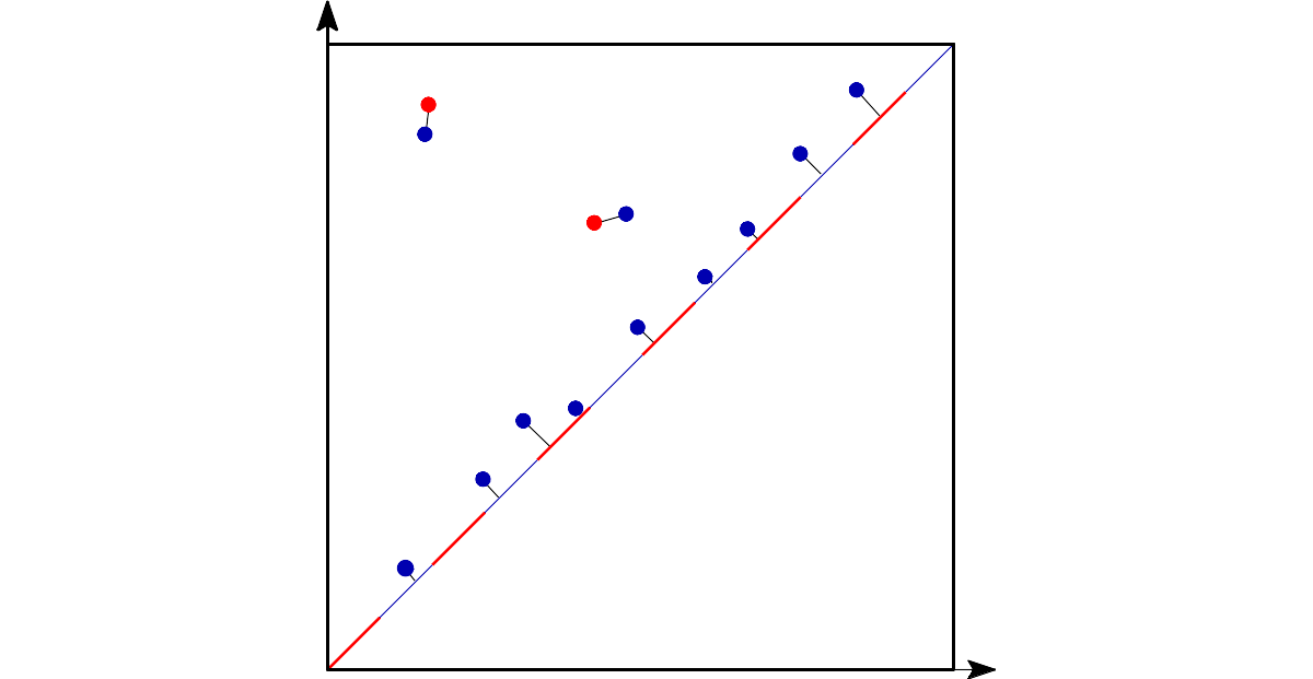
If we track the birth and death (when they die when they merge with an older component) of the homology classes as a pairs $(b,d)$, we can draw these pairs in two dimensions to obtain a persistence diagram.

A persistence diagrams can be considered like a signature of the dataset, and these signatures can be compared. Different distances can be defined between persistence diagrams. One of them is the bottleneck distance defined as the infimum of the supremum of the infinity norms of all possible bijections between the persistence diagrams.

You may wonder why we are introducing all these concepts of persistent homology. The reason is that the $\epsilon$ is difficult to compute and by $\epsilon$ I mean the representativeness parameter. However, it can be upper and lower bounded by the bottleneck distance and the Hausdorff distance. Specifically, half of the bottleneck distance between the persistence diagrams are a lower bound and the Hausdorff distance is an upper bound. The value of the representativeness dataset is equal to the Gromov-Hausdorff distance between the sets (but is hard to compute!). So, once we are given a dataset and we want to check how representative is from another, we can use these two measures to bound and approximate the representativeness.

Conclusions

There are a lot more to do, but there are strong results for the perceptron case. However, even if it may be difficult to build a general theory for any kind of architecture (might be impossible), I think it could be approachable and interesting to find the effects of reducing datasets for different architectures to get a better time of the training execution and even reduce the needed storage. Furthermore, it might have applications to the unbalance problem for classification tasks, and so on. As usual, for a more technical approach to this post theme, you can check the papers.