In this post, I would like to describe a little bit our first approach to give a constructive solution to the Universal Approximation theorem. This approach is developed in a formal taste in the following preprint: “Two-hidden-layer Feedforward Neural Networks are Universal Approximators: A Constructive Approach”.

Those who have studied a little about Machine Learning, and Artificial Neural Networks (ANNs) should know about the Universal Approximation theorem. It states, roughly speaking, that an ANN with only one hidden layer can approximate any continuous function (with some constraints), as closely as we desired. The traditional proofs were based in existence arguments, i.e. these proofs state that there is one but with no clue about how many neurons (or units) the ANN should have in the hidden layer.

So, let us begin with an informal introduction to this Universal Approximation theorem and our version of it. We did not pretend to solve it, but we restricted ourselves to a smaller version of it, and, using simplicial complexes, we gave this constructive version of the proof.

Artificial Neural Networks

Artificial Neural Networks can be described as computational graphs which are directed and have weights. These weights are usually updated in a training process, trying to solve an optimization problem. This optimization problem is based on a function that measures how far is the model (i.e. the ANN) from the right classification of a dataset. In our case, we will not use any kind of training, but we will give, as we will explain below, the specific values for the weights.

As we were explaining, an ANN is a computational graph. However, the Universal Approximation theorem traditionally restricts to the case of one hidden layer ANNs.

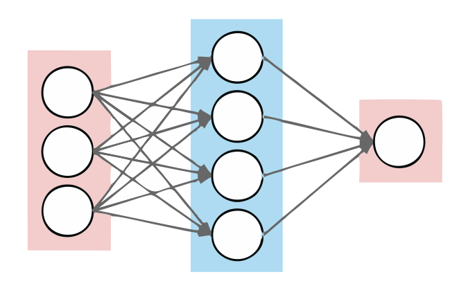
As we can see in the picture, there are three layers of neurons, the first layer is an input layer, the second one is the so-called hidden layer, and the last one is the output layer. This ANNs can be written in a mathematical formula by $F(x)=\sum_{i=1}^{N} v_{i} \varphi\left(w_{i}^{T} x+b_{i}\right)$ where $\varphi$ is an activation function, $b_i$ is the bias term, and $w_i$ are the weights. The Universal Approximation theorem claims that any continuous function from a compact to $\mathbb{R}$ can be approximated by one of these ANNs with just one hidden layer. However, as mentioned above, there is no clue about how many neurons must compose the hidden layer.

In our case, we will get a more difficult ANN architecture. We will use two hidden layers that will have a very specific commitment. The idea is very simple: having a triangulation of a given space, we will obtain its barycentric coordinates with the first hidden layer. Then, in the second hidden layer, we will approximate the continuous function by a simplicial approximation (whatever it is, we will explain below). Then, we recover the cartesian coordinates. In our case, we can approximate any continuous function from a space $X$ to a space $Y$. However, it is important for us that both spaces are triangulable. Besides, sometimes it is not easy to get such a triangulation.

Simplicial Complexes

Simplicial complexes will be our main structure (¹). If we want to approximate a continuous function from a given space $X\subset \mathbb{R}^n$ to $Y\subset \mathbb{R}^m$, we need a more simple representation of $X$ and $Y$. So, if $X$ and $Y$ are triangulable, and we know that triangulation, we can build a continuous function that approximates the original continuous function.

A simplicial complex $K$ is (roughly speaking) a data structure that is built by gluing small pieces called simplices: $0$-simplices are points, $1$-simplices are edges, $2$-simplices are triangles, $3$-simplices are tetrahedrons, and so on. This data structure is widely used to represent topological spaces. However, not all spaces are triangulable.

Let us assume that we have two triangulable spaces $X$ and $Y$, and a continuous function $g:X\rightarrow Y$. Then, we could obtain two simplicial complexes $K$ and $L$ from $X$ and $Y$, respectively. The question now is, how can we define a function between these two simplicial complexes?

Maps between simplicial complexes are called simplicial maps. They are defined from simplices of a simplicial complex to simplices of another (or the same) simplicial complex. Then, it can be extended to a continuous function by $\sum_{i=0}^n b_i(x)\phi(u_i)$ where $b_i(x)$ are the barycentric coordinates of $x$, and $\phi$ is the map defined between vertices of simplicial complexes.

Besides, there exists a simplicial approximation theorem that states: for any continuous function there exists a simplicial approximation. However, barycentric subdivision of the given triangulations are needed to satisfy the conditions of the theorem. We can take the following example from (Edelsbrunner et. al).

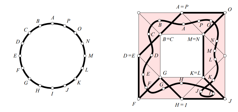
In this image, we can see two simplicial complexes, one describing a circumference, and another circular crown alike. Then, a continuous deformation is done to the circumference, and it is embedded into the simplicial complex at the right. Finally, it is approximated by the simplicial approximation. However, in most cases, the barycentric subdivision will be needed to satisfy a star condition in the domain simplicial complex.

In our case, we need to do barycentric subdivision to both simplicial complexes. The reason is that we desire to get a tight approximation of a continuous function. Therefore, we need to get a tight mesh in the image simplicial complex, having then a closer simplicial approximation. Let us summarize:

Having two triangulable spaces $X$ and $Y$. We can obtain two triangulations $K$ and $L$ of $X$ and $Y$, respectively. Then, if we want to approximate a continuous function $g:X\rightarrow Y$, we can find $t_1$ and $t_2$ such that $f:Sd^{t_1}K\rightarrow Sd^{t_2}L$ is a simplicial approximation of $g$, and it is as close as we want. Where $Sd^t$ denotes the $t$-th barycentric subdivision.

Finally, we should translate this simplicial approximation to a two hidden neural network.

Two hidden neural network and simplicial maps

At this point, you might have an idea of what the relationship between ANN and simplicial map is. Once we have a simplicial map, that is a simplicial approximation of a given continuous function, we can translate it into two hidden layers.

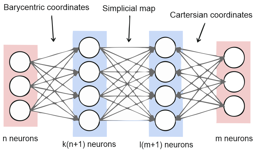
We are assuming here that the input data is $n$-dimensional. Then, the first hidden layer receives the barycentric coordinates of the input data, but for each maximal simplex of the input triangulation. The next hidden layer receives the output of the simplicial map in barycentric coordinates. Finally, the output layer combine these coordinates to cartesian coordinates with the following activation function $\frac{\sum_{j=1}^{\ell} z_{j} \psi\left(y_{j}\right)}{\sum_{j=1}^{\ell} y_{j}}$ where $\psi(y_j)=1$ if all the coordinates of $y_j$ are equal to or greater than $0$. This last activation function combines all the barycentric coordinates of each maximal simplex of the image simplicial complex.

Therefore, to compute the weights is not needed to do any kind of training but determine the right matrices and bias terms to do the coordinates transformations. Besides, the weights between the first and second hidden layer are clearly determined by the simplicial map.

Conclusions

This research tries to give a constructive approach to a version of the Universal Approximation theorem. However, we had to use a deeper architecture than the one used by this theorem, and restrict the case of study to triangulable spaces. I hope you enjoyed this post, and remember that for references or a more formal explanation of the topic you can check the paper on arXiv.